This is the one of the basic test cases, also the first case for understanding SPH method for non-Newtonian low Reynolds number flows.
Example 17: 2D throat
As shown in the figure, the schematic sketch of the initial setup.
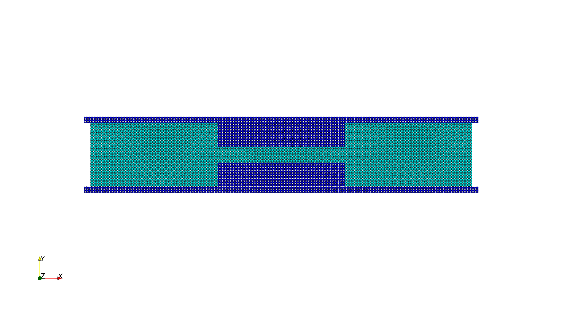
Initial configuration
First, we provide the parameters for geometric modeling and numerical setup.
#include "sphinxsys.h"
using namespace SPH;

Real DH = 4.0;                                  //channel height
Real DT = 1.0;                                  //throat height
Real DL = 24.0;                                 //channel length
Real resolution_ref = 0.1;              //particle spacing
Real BW = resolution_ref * 4.0; //boundary width
/** Domain bounds of the system. */
BoundingBox system_domain_bounds(Vec2d(-0.5 * DL - BW, -0.5 * DH - BW),
                                                                 Vec2d(0.5 * DL + BW, 0.5 * DH + BW));
DH is the channel height,
DT is the throat height,
DL is the channel length,
resolution_ref gives the reference of initial particle spacing,
BW gives the boundary width,
system_domain_bounds defines the domain of this case.
Then we give the material properties.
Real rho0_f = 1.0;
Real gravity_g = 1.0;     /**< Gravity force of fluid. */
Real Re = 0.001;                  /**< Reynolds number defined in the channel */
Real mu_f = rho0_f * sqrt(0.5 * rho0_f * powerN(0.5 * DH, 3) * gravity_g / Re);
Real U_c = 0.5 * powerN(0.5 * DH, 2) * gravity_g * rho0_f / mu_f;
Real U_f = U_c * DH / DT;
Real c_f = 10.0 * (U_f, sqrt(mu_f / rho0_f * U_f / DT));
Real mu_p_f = 0.6 * mu_f;
Real lambda_f = 10.0;
rho0_f is the density of the fluid,
gravity_g is gravity force of fluid,
Re is Reynolds number defined in the channel,
mu_f is viscosity,
U_c is the maximum velocity in the channel,
U_f is the maximum velocity in the throat,
c_f is the sound of speed,
mu_p_f is the polymeric viscosity,
lambda_f is the relaxation time,
and in this case, all parameters are non-dimensional.
Here, we create the fluid and wall bodies.
//----------------------------------------------------------------------
// Create fluid body
//----------------------------------------------------------------------
class FluidBlock : public FluidBody
{
public:
        FluidBlock(SPHSystem &system, const std::string &body_name)
                : FluidBody(system, body_name)
        {
                std::vector<Vecd> pnts;
                pnts.push_back(Vecd(-0.5 * DL, -0.5 * DH));
                pnts.push_back(Vecd(-0.5 * DL, 0.5 * DH));
                pnts.push_back(Vecd(-DL / 6.0, 0.5 * DH));
                pnts.push_back(Vecd(-DL / 6.0, -0.5 * DH));
                pnts.push_back(Vecd(-0.5 * DL, -0.5 * DH));

                std::vector<Vecd> pnts1;
                pnts1.push_back(Vecd(-DL / 6.0 - BW, -0.5 * DT));
                pnts1.push_back(Vecd(-DL / 6.0 - BW, 0.5 * DT));
                pnts1.push_back(Vecd(DL / 6.0 + BW, 0.5 * DT));
                pnts1.push_back(Vecd(DL / 6.0 + BW, -0.5 * DT));
                pnts1.push_back(Vecd(-DL / 6.0 - BW, -0.5 * DT));

                std::vector<Vecd> pnts2;
                pnts2.push_back(Vecd(DL / 6.0, -0.5 * DH));
                pnts2.push_back(Vecd(DL / 6.0, 0.5 * DH));
                pnts2.push_back(Vecd(0.5 * DL, 0.5 * DH));
                pnts2.push_back(Vecd(0.5 * DL, -0.5 * DH));
                pnts2.push_back(Vecd(DL / 6.0, -0.5 * DH));

                MultiPolygon multi_polygon;
                multi_polygon.addPolygon(pnts, ShapeBooleanOps::add);
                multi_polygon.addPolygon(pnts1, ShapeBooleanOps::add);
                multi_polygon.addPolygon(pnts2, ShapeBooleanOps::add);

                body_shape_.add<MultiPolygonShape>(multi_polygon);
        }
};

//----------------------------------------------------------------------
// Create wall body
//----------------------------------------------------------------------
class WallBoundary : public SolidBody
{
public:
        WallBoundary(SPHSystem &system, const std::string &body_name)
                : SolidBody(system, body_name)
        {
                std::vector<Vecd> pnts3;
                pnts3.push_back(Vecd(-0.5 * DL - BW, -0.5 * DH - BW));
                pnts3.push_back(Vecd(-0.5 * DL - BW, 0.5 * DH + BW));
                pnts3.push_back(Vecd(0.5 * DL + BW, 0.5 * DH + BW));
                pnts3.push_back(Vecd(0.5 * DL + BW, -0.5 * DH - BW));
                pnts3.push_back(Vecd(-0.5 * DL - BW, -0.5 * DH - BW));

                std::vector<Vecd> pnts;
                pnts.push_back(Vecd(-0.5 * DL - 2.0 * BW, -0.5 * DH));
                pnts.push_back(Vecd(-0.5 * DL - 2.0 * BW, 0.5 * DH));
                pnts.push_back(Vecd(-DL / 6.0, 0.5 * DH));
                pnts.push_back(Vecd(-DL / 6.0, -0.5 * DH));
                pnts.push_back(Vecd(-0.5 * DL - 2.0 * BW, -0.5 * DH));

                std::vector<Vecd> pnts1;
                pnts1.push_back(Vecd(-DL / 6.0 - BW, -0.5 * DT));
                pnts1.push_back(Vecd(-DL / 6.0 - BW, 0.5 * DT));
                pnts1.push_back(Vecd(DL / 6.0 + BW, 0.5 * DT));
                pnts1.push_back(Vecd(DL / 6.0 + BW, -0.5 * DT));
                pnts1.push_back(Vecd(-DL / 6.0 - BW, -0.5 * DT));

                std::vector<Vecd> pnts2;
                pnts2.push_back(Vecd(DL / 6.0, -0.5 * DH));
                pnts2.push_back(Vecd(DL / 6.0, 0.5 * DH));
                pnts2.push_back(Vecd(0.5 * DL + 2.0 * BW, 0.5 * DH));
                pnts2.push_back(Vecd(0.5 * DL + 2.0 * BW, -0.5 * DH));
                pnts2.push_back(Vecd(DL / 6.0, -0.5 * DH));

                MultiPolygon multi_polygon;
                multi_polygon.addPolygon(pnts3, ShapeBooleanOps::add);
                multi_polygon.addPolygon(pnts, ShapeBooleanOps::sub);
                multi_polygon.addPolygon(pnts1, ShapeBooleanOps::sub);
                multi_polygon.addPolygon(pnts2, ShapeBooleanOps::sub);

                body_shape_.add<MultiPolygonShape>(multi_polygon);
        }
};
After completing the initial geometric modeling and numerical setup, we come to the int main() function.
SPHSystem system(system_domain_bounds, resolution_ref);

GlobalStaticVariables::physical_time_ = 0.0;

In_Output in_output(system);
In the first part of main function, an object of SPHSystem is created, the starting time GlobalStaticVariables::physical_time_ = 0.0 and outout enviroment In_Output in_output(system) are set.
Then create body, materials and particles for fluid channel and solid wall
FluidBlock fluid_block(system, "FluidBody");
ViscoelasticFluidParticles fluid_particles(fluid_block, makeShared<Oldroyd_B_Fluid>(rho0_f, c_f, mu_f, lambda_f, mu_p_f));

WallBoundary wall_boundary(system, "Wall");
SolidParticles wall_particles(wall_boundary);
Oldroyd_B_Fluid is a non-Newtonian flow material.
Define the contact map.
BodyRelationInner fluid_block_inner(fluid_block);
ComplexBodyRelation fluid_block_complex(fluid_block_inner, {&wall_boundary});
Using class BodyRelationInner means beam_body_inner defines the inner data connections.
And using class ComplexBodyRelation means the relation combined an inner and a contactbody relation.
Define outputs functions
BodyStatesRecordingToVtp write_real_body_states(in_output, system.real_bodies_);
Then the main algorithm is defined, including the general methods: time stepping based on fluid dynamics, fluid dynamics and boundary conditions.
PeriodicConditionInAxisDirectionUsingGhostParticles periodic_condition(fluid_block, xAxis);
//evaluation of density by summation approach
fluid_dynamics::DensitySummationComplex update_density_by_summation(fluid_block_complex);
//time step size without considering sound wave speed and viscosity
fluid_dynamics::AdvectionTimeStepSizeForImplicitViscosity get_fluid_advection_time_step_size(fluid_block, U_f);
//time step size with considering sound wave speed
fluid_dynamics::AcousticTimeStepSize get_fluid_time_step_size(fluid_block);
//pressure relaxation using verlet time stepping
fluid_dynamics::PressureRelaxationWithWallOldroyd_B pressure_relaxation(fluid_block_complex);
pressure_relaxation.pre_processes_.push_back(&periodic_condition.ghost_update_);
fluid_dynamics::DensityRelaxationWithWallOldroyd_B density_relaxation(fluid_block_complex);
density_relaxation.pre_processes_.push_back(&periodic_condition.ghost_update_);
//define external force
Gravity gravity(Vecd(gravity_g, 0.0));
TimeStepInitialization initialize_a_fluid_step(fluid_block, gravity);
fluid_dynamics::ViscousAccelerationWithWall viscous_acceleration(fluid_block_complex);
//computing viscous effect implicitly and with update velocity directly other than viscous acceleration
DampingPairwiseWithWall<Vec2d, DampingPairwiseInner>
        implicit_viscous_damping(fluid_block_complex, "Velocity", mu_f);
//impose transport velocity
fluid_dynamics::TransportVelocityCorrectionComplex transport_velocity_correction(fluid_block_complex);
//computing vorticity in the flow
fluid_dynamics::VorticityInner compute_vorticity(fluid_block_inner);
PeriodicConditionInAxisDirectionUsingGhostParticles : to impose the perodic condintion on the inlet and outlet.
DensitySummationComplex : to compute density through summation approch.
AdvectionTimeStepSizeForImplicitViscosity : to compute the advection time step size.
AcousticTimeStepSize : to compute acoustic time step size.
PressureRelaxationWithWallOldroyd_B : to compute the acceleration due to the elastic force.
DensityRelaxationWithWallOldroyd_B : to compute the change rate of elastic stress and elastic stress.
ViscousAccelerationWithWall : to compute the viscous acceleration.
DampingPairwiseWithWall : a quantity damping by a pairwise splitting scheme.
TransportVelocityCorrectionComplex : to eliminate the tensile instability.
VorticityInner : to compute the vorticity of the flow.
Initialization includes cell linked lists and configuration for bodies and surface normal direction.
system.initializeSystemCellLinkedLists();
//initial periodic boundary condition
periodic_condition.ghost_creation_.parallel_exec();
system.initializeSystemConfigurations();
//prepare quantities will be used once only
wall_particles.initializeNormalDirectionFromBodyShape();
Finally, the time-stepping loop.
int number_of_iterations = 0;
int screen_output_interval = 100;
Real End_Time = 5;
Real D_Time = 0.01; //time step size for ouput file
Real dt = 0.0;     //default acoustic time step sizes
//statistics for computing time
tick_count t1 = tick_count::now();
tick_count::interval_t interval;
//----------------------------------------------------------------------
//      First output before the main loop.
//----------------------------------------------------------------------
write_real_body_states.writeToFile();
//----------------------------------------------------------------------
//      Main loop starts here.
//----------------------------------------------------------------------
while (GlobalStaticVariables::physical_time_ < End_Time)
{
        Real integration_time = 0.0;
        //integrate time (loop) until the next output time
        while (integration_time < D_Time)
        {

                initialize_a_fluid_step.parallel_exec();
                Real Dt = get_fluid_advection_time_step_size.parallel_exec();
                update_density_by_summation.parallel_exec();
                transport_velocity_correction.parallel_exec(Dt);

                Real relaxation_time = 0.0;
                while (relaxation_time < Dt)
                {
                        dt = SMIN(get_fluid_time_step_size.parallel_exec(), Dt);
                        implicit_viscous_damping.parallel_exec(dt);
                        pressure_relaxation.parallel_exec(dt);
                        density_relaxation.parallel_exec(dt);

                        relaxation_time += dt;
                        integration_time += dt;
                        GlobalStaticVariables::physical_time_ += dt;
                }

                if (number_of_iterations % screen_output_interval == 0)
                {
                        std::cout << std::fixed << std::setprecision(9) << "N=" << number_of_iterations << "    Time = "
                                          << GlobalStaticVariables::physical_time_
                                          << "  Dt = " << Dt << "       dt = " << dt << "\n";
                }
                number_of_iterations++;

                //water block configuration and periodic condition
                periodic_condition.bounding_.parallel_exec();
                fluid_block.updateCellLinkedList();
                periodic_condition.ghost_creation_.parallel_exec();
                fluid_block_complex.updateConfiguration();
        }

        tick_count t2 = tick_count::now();
        compute_vorticity.parallel_exec();
        write_real_body_states.writeToFile();
        tick_count t3 = tick_count::now();
        interval += t3 - t2;
}
tick_count t4 = tick_count::now();

tick_count::interval_t tt;
tt = t4 - t1 - interval;
std::cout << "Total wall time for computation: " << tt.seconds() << " seconds." << std::endl;

return 0;
periodic_condition.bounding_.parallel_exec(), fluid_block.updateCellLinkedList(),
periodic_condition.ghost_creation_.parallel_exec() and fluid_block_complex.updateConfiguration() means
the cell link list and configuration need to be updated every Dt time step.
During the looping, outputs are scheduled. On screen output will be the number of time steps, the current physical time and acoustic time-step size. After the simulation is terminated, the statistics of computation time are outputed to the screen. Note that the total computation time has excluded the time for writing files.
After the simulation process, you can use the Paraview to read the result files. The following figure shows the velocity field.
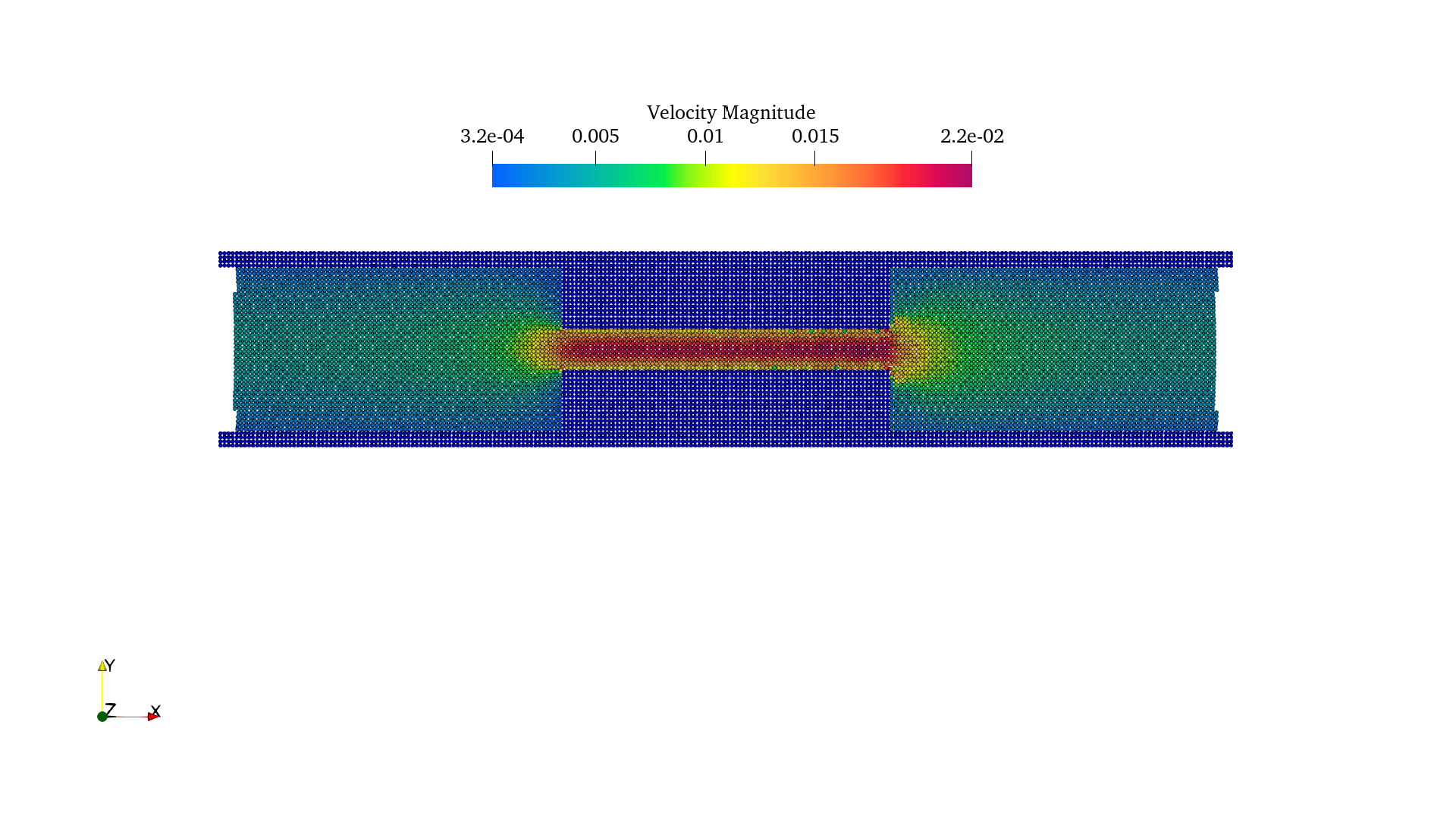
The velocity field of throat.